13 Chapter 12: Diffusion Models
14 The Unifying Story: DAE + VAE = Diffusion
14.1 The Core Narrative
Diffusion models emerged from the marriage of two seemingly disparate ideas:
Denoising Autoencoders (DAE): Learn to remove noise from data, capturing local geometry via the score function (\(\nabla_x \log p(x)\))
Variational Autoencoders (VAE): Model data by learning to decode from a global iid noise prior \(\mathcal{N}(0,I)\)
The fundamental tension:
DAE works with small noise → learns local structure but cannot sample globally
VAE assumes full noise → reaches iid prior easily but requires compression bottleneck, loses fidelity
Diffusion’s insight: Bridge the gap by gradually adding noise across many steps, making each step a well-conditioned local denoising problem, while collectively reaching full iid noise.
One-Line Summary:
Diffusion models are VAEs whose decoder is implemented as a continuous family of denoising autoencoders across noise scales.
15 Denoising Autoencoders: The Foundation
15.1 Classical DAE (Vincent et al., 2008–2011)
Training objective: \[\mathcal{L}_{\text{DAE}} = \mathbb{E}_{x \sim p_{\text{data}},\, \epsilon \sim \mathcal{N}(0,\sigma^2 I)} \big[\|f_\theta(x + \epsilon) - x\|^2\big]\]
Procedure:
Corrupt data slightly: \(\tilde{x} = x + \epsilon\)
Learn to reconstruct: \(f_\theta(\tilde{x}) \approx x\)
15.2 Connection to Score Functions
Key theoretical result (Vincent 2011):
As \(\sigma \to 0\), the optimal denoiser satisfies: \[f_\theta(x) - x \;\propto\; \nabla_x \log p(x)\]
Key insight: DAE learns the score (gradient of log density).
What is the score function?
The score function \(\nabla_x \log p(x)\) is the gradient of the log probability density with respect to the data \(x\). It tells you which direction to move in data space to increase the probability.
Points "uphill" toward regions of higher probability density
At high-probability regions (e.g., real images): score is small (already at peak)
At low-probability regions (e.g., noise): score points strongly toward real data
The data score \(\nabla_x \log p_{\text{data}}(x)\) specifically refers to the score of the true data distribution
Why it matters: Denoising is equivalent to following this gradient to remove corruption – the denoiser learns to point from noisy samples back toward the data manifold.
Simplified proof intuition:
Consider corrupted data \(\tilde{x} = x + \epsilon\) where \(\epsilon \sim \mathcal{N}(0, \sigma^2 I)\). The optimal denoiser minimizes: \[\mathbb{E}_{p(x)} \mathbb{E}_{\epsilon}[\|f_\theta(\tilde{x}) - x\|^2]\]
Taking the gradient with respect to \(f_\theta(\tilde{x})\) and setting to zero: \[f_\theta(\tilde{x}) = \mathbb{E}[x | \tilde{x}]\]
By Tweedie’s formula, for Gaussian noise: \[\mathbb{E}[x | \tilde{x}] = \tilde{x} + \sigma^2 \nabla_{\tilde{x}} \log p(\tilde{x})\]
Therefore: \[f_\theta(\tilde{x}) - \tilde{x} = \sigma^2 \nabla_{\tilde{x}} \log p(\tilde{x})\]
Key takeaway: The denoising direction is exactly the score function \(\nabla \log p(\tilde{x})\) scaled by \(\sigma^2\). As \(\sigma \to 0\), the corrupted distribution converges to the clean data distribution: \(p(\tilde{x}) \to p_{\text{data}}(x)\). Therefore, denoising directly estimates the data score \(\nabla_x \log p_{\text{data}}(x)\) – the gradient of the log probability of the true data distribution.
Connection to MCMC: Reverse-Time Fixed Points
Recall from MCMC (Part 1): we construct Markov operators whose stationary distribution is the target \(\pi(x)\). The forward diffusion process has a similar structure:
Forward process: \(q(x_t \mid x_{t-1})\) gradually adds noise, with stationary distribution \(\mathcal{N}(0, I)\)
Reverse process: \(p_\theta(x_{t-1} \mid x_t)\) removes noise, with stationary distribution \(p_{\text{data}}(x_0)\)
The key difference: MCMC uses detailed balance to maintain equilibrium at a single distribution, while diffusion uses time-reversed dynamics to construct a path between two distributions (\(\mathcal{N}(0,I) \to p_{\text{data}}\)).
Score matching is the reverse-process analog of acceptance ratios in Metropolis-Hastings–it ensures the reverse dynamics correctly invert the forward process by learning \(\nabla \log p_t(x_t)\) at each timestep.
Both MCMC and diffusion are fundamentally about designing stochastic dynamics with desired equilibrium properties. MCMC: single fixed point. Diffusion: trajectory between fixed points.
15.3 Manifold Learning with DAE
The manifold hypothesis: Natural data (images, text) lies on a low-dimensional manifold embedded in high-dimensional space. A denoising autoencoder learns this manifold structure:
Corruption: Adding noise pushes data points off the manifold
Denoising: The DAE learns to project corrupted points back onto the data manifold
Learned geometry: By training on multiple corruption levels, the DAE implicitly discovers the manifold’s local tangent space structure
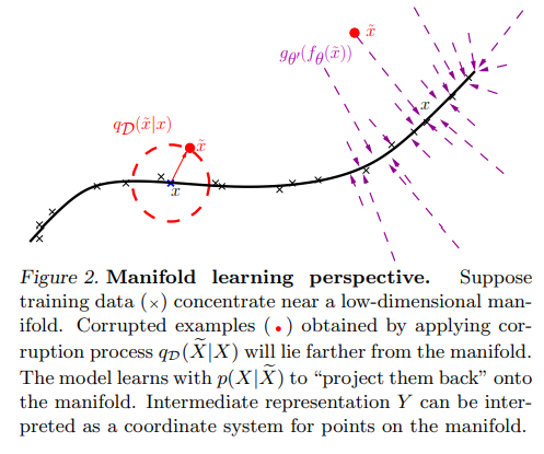
Why this matters for diffusion: Multi-scale manifold learning (applying denoising at different noise levels) is why diffusion produces such high-quality samples–it learns the data geometry at every scale from global structure to fine details.
15.4 Why Plain DAE Fails
The small-noise limitation:
Small noise (\(\sigma\) small): Only learns local geometry → cannot sample globally
Large noise (\(\sigma\) large): Denoising becomes ill-posed → one network cannot map pure noise \(\to\) data
This is the fundamental problem diffusion solves.
16 VAE: The Global Prior Perspective
16.1 VAE’s Contrasting Approach
VAE assumes a global latent code with iid prior: \[z \sim \mathcal{N}(0, I)\]
And learns: \[\begin{align} q_\phi(z|x) & \quad \text{(encoder)} \\ p_\theta(x|z) & \quad \text{(decoder)} \end{align}\]
16.2 VAE Training: The ELBO
The problem: We want to maximize \(\log p(x)\), but computing \(p(x) = \int p_\theta(x|z)p(z)dz\) is intractable.
The solution: Use variational inference with approximate posterior \(q_\phi(z|x)\). Starting from: \[\log p(x) = \log \int p_\theta(x|z)p(z)dz\]
Multiply and divide by \(q_\phi(z|x)\): \[\log p(x) = \log \mathbb{E}_{q_\phi(z|x)}\left[\frac{p_\theta(x|z)p(z)}{q_\phi(z|x)}\right]\]
By Jensen’s inequality (\(\log \mathbb{E}[X] \ge \mathbb{E}[\log X]\)): \[\log p(x) \ge \mathbb{E}_{q_\phi(z|x)}\left[\log \frac{p_\theta(x|z)p(z)}{q_\phi(z|x)}\right]\]
Rearranging: \[\log p(x) \ge \mathbb{E}_{q_\phi(z|x)}[\log p_\theta(x|z)] - \text{KL}(q_\phi(z|x) \| p(z))\]
This is the Evidence Lower Bound (ELBO). It consists of:
Reconstruction term: \(\mathbb{E}_{q_\phi(z|x)}[\log p_\theta(x|z)]\) – how well decoder reconstructs \(x\) from \(z\)
Regularization term: \(\text{KL}(q_\phi(z|x) \| p(z))\) – keeps encoder’s posterior close to prior
Training: Maximize ELBO jointly over \(\theta\) (decoder) and \(\phi\) (encoder) using reparameterization trick.
16.3 VAE’s Limitations
+ Reaches iid noise easily
+ Enables global sampling
- Requires compression bottleneck
- Blurry reconstructions (due to single-step decode)
17 Diffusion Models: The Synthesis
17.1 The Key Insight
Core Idea:
What if we keep DAE’s denoising principle, but make noise large by decomposing it into infinitesimal steps – and wrap it in a variational model?
This is exactly diffusion.
17.2 Forward Process: Gradual Noise Addition
Fixed corruption schedule: \[x_t = \sqrt{\alpha_t}\, x_0 + \sqrt{1-\alpha_t}\, \epsilon, \quad \epsilon \sim \mathcal{N}(0,I)\]
where \(\alpha_t \in [0,1]\) decreases with \(t\).
As \(t \to T\): \[x_T \sim \mathcal{N}(0, I)\]
This solves the "large noise" problem by gradual destruction.
Diffusion schedule example (1000 steps):
\(t=0\): \(\alpha_0 = 1\) → \(x_0\) = original image
\(t=250\): \(\alpha_{250} = 0.85\) → slight blur
\(t=500\): \(\alpha_{500} = 0.5\) → heavy noise
\(t=1000\): \(\alpha_{1000} \approx 0\) → pure Gaussian noise
17.3 Reverse Process: Multi-Scale Denoising
Learn to reverse each step: \[p_\theta(x_{t-1} | x_t) = \mathcal{N}(x_{t-1}; \mu_\theta(x_t, t), \Sigma_\theta(x_t, t))\]
Each step is a small-noise DAE:
Easy to learn (well-conditioned)
Local denoising
Indexed by noise level \(t\)
Key insight: Diffusion is a continuum of DAEs indexed by noise level.
17.4 Training Objective: The Variational Connection
Diffusion training optimizes an ELBO: \[\log p(x_0) \ge \sum_{t=1}^T \mathbb{E}[\log p_\theta(x_{t-1}|x_t)] - \text{KL}(q(x_T|x_0) \| p(x_T))\]
Interpretation:
Latents: \(x_1, x_2, \ldots, x_T\) (entire noise trajectory)
Prior: \(p(x_T) = \mathcal{N}(0,I)\)
Encoder: Fixed (forward diffusion)
Decoder: Learned (denoising steps)
Diffusion = Hierarchical VAE
This is not metaphorical – it is exact. Diffusion is a VAE where:
The latent space is the entire noise trajectory
The encoder is fixed (forward diffusion process)
The decoder is learned (reverse denoising process)
17.5 Simplified Training Loss (Ho et al., 2020)
In practice, the ELBO simplifies to: \[\mathcal{L}_{\text{simple}} = \mathbb{E}_{t, x_0, \epsilon}\big[\|\epsilon - \epsilon_\theta(x_t, t)\|^2\big]\]
where \(\epsilon_\theta\) is a neural network predicting the noise \(\epsilon\) from noisy input \(x_t\).
Training procedure:
Sample \(x_0 \sim p_{\text{data}}\), \(t \sim \text{Uniform}(1, T)\), \(\epsilon \sim \mathcal{N}(0,I)\)
Compute \(x_t = \sqrt{\alpha_t} x_0 + \sqrt{1-\alpha_t} \epsilon\)
Train \(\epsilon_\theta\) to predict \(\epsilon\) from \(x_t\) and \(t\)
PyTorch training loop (simplified):
def train_step(x0, model, t_max=1000):
t = torch.randint(0, t_max, (x0.shape[0],))
noise = torch.randn_like(x0)
alpha_t = get_alpha(t) # schedule
x_t = sqrt(alpha_t) * x0 + sqrt(1 - alpha_t) * noise
pred_noise = model(x_t, t)
loss = F.mse_loss(pred_noise, noise)
return loss
17.6 Sampling: Iterative Denoising
Generation procedure:
Start from pure noise: \(x_T \sim \mathcal{N}(0, I)\)
For \(t = T, T-1, \ldots, 1\):
Predict noise: \(\epsilon_\theta(x_t, t)\)
Denoise one step: \(x_{t-1} = \frac{1}{\sqrt{\alpha_t}}(x_t - \frac{1-\alpha_t}{\sqrt{1-\bar{\alpha}_t}} \epsilon_\theta(x_t, t)) + \sigma_t z\)
Return \(x_0\) (generated sample)
18 Architectures in Practice
18.1 U-Net: The Standard Backbone
Architecture:
Encoder-decoder with skip connections
Time embedding \(t\) injected at each block
Self-attention at lower resolutions
Residual blocks with GroupNorm
Why U-Net?
Skip connections preserve high-frequency details
Multi-scale processing matches multi-scale noise
Efficient for images
18.2 Transformer-Based: Diffusion Transformers (DiT)
DiT (Peebles & Xie, 2023):
Replace U-Net with Vision Transformer
Patch-based input (like ViT)
Conditional via adaptive layer norm (adaLN)
Scales better than U-Net (compute vs quality)
When to use DiT vs U-Net:
U-Net: Images, faster inference, lower compute
DiT: High resolution, large-scale training, better scaling laws
19 Practical Models and Applications
19.1 Text-to-Image: Stable Diffusion
Key innovation: Latent diffusion (Rombach et al., 2022)
Architecture:
VAE encoder: \(z = \mathcal{E}(x)\) (compress \(512 \times 512\) to \(64 \times 64\))
Diffusion in latent space: \(z_t = \sqrt{\alpha_t} z + \sqrt{1-\alpha_t} \epsilon\)
U-Net with cross-attention to CLIP text embeddings
VAE decoder: \(\hat{x} = \mathcal{D}(z_0)\)
Why latent space?
+ \(8 \times\) compute reduction (vs pixel space)
+ Faster sampling (50 steps \(\sim\)5 seconds on GPU)
+ Still high fidelity
19.2 Other Production Models
| Model | Organization | Key Feature |
|---|---|---|
| DALL-E 2 | OpenAI | CLIP guidance, unCLIP decoder |
| Imagen | Cascaded diffusion, T5 text encoder | |
| Midjourney | Midjourney | Proprietary, aesthetic fine-tuning |
| Stable Diffusion | Stability AI | Open source, latent diffusion |
| Stable Diffusion 3 | Stability AI | Rectified flow, improved text rendering |
19.3 Where Diffusion Excels
Visual generation (images, video):
Photo-realistic images (beats GANs on fidelity)
Fine detail preservation (high-frequency content)
Controllability (text, sketch, depth, pose)
Audio (speech, music):
WaveGrad (speech synthesis)
Diff-SVC (singing voice conversion)
Riffusion (music generation from text)
3D and motion:
DreamFusion (text-to-3D via score distillation)
MDM (human motion diffusion)
When NOT to use diffusion:
Real-time applications (slow sampling)
Low-dimensional data (overkill)
Discrete data (text) – autoregressive models better
20 Key Developments Timeline
2008–2011: Denoising Autoencoders (Vincent et al.) – score matching connection
2015: Diffusion Probabilistic Models (Sohl-Dickstein et al.) – forward/reverse process formulation
2019: Score-Based Generative Models (Song & Ermon) – Langevin dynamics, annealed noise
2020: DDPM (Ho et al.) – simplified loss, practical training
2021: Score SDEs (Song et al.) – continuous-time limit, probability flow ODE
2021: Guided Diffusion (Dhariwal & Nichol) – classifier guidance, beats GANs on ImageNet
2022: Stable Diffusion (Rombach et al.) – latent diffusion, open source explosion
2022: DALL-E 2, Imagen – production text-to-image systems
2023: Consistency Models (Song et al.) – single-step generation
2024: Rectified Flow/Flow Matching – deterministic trajectories, faster sampling
21 Interview Cheat Phrases
“Diffusion models are VAEs whose decoder is a continuous family of denoising autoencoders across noise scales.”
“DAEs learn local geometry via score matching, VAEs assume global iid priors – diffusion bridges them with gradual noise addition.”
“Training is simple: corrupt data to random timestep, predict noise, MSE loss. Sampling is iterative denoising from pure noise.”
“Latent diffusion (Stable Diffusion) runs diffusion in VAE latent space – 8× faster, same quality.”
“Diffusion beats GANs on fidelity but is slower at inference – typical trade-off is 50 steps vs 1 forward pass.”
“U-Net is standard for images (skip connections, multi-scale). DiT (transformer) scales better for large models.”
“Key papers: DDPM (2020) for practical training, Score SDEs (2021) for theory, Stable Diffusion (2022) for production.”
Common Interview Question: How does diffusion differ from VAE?
Both are likelihood-based generative models with variational objectives. VAE learns a single compressed latent \(z\) and decodes in one shot – fast but blurry. Diffusion learns a sequence of latents \(x_1, \ldots, x_T\) representing noise levels, with a fixed encoder (forward diffusion) and learned decoder (reverse denoising). This hierarchical structure enables higher fidelity at the cost of iterative sampling.
22 Practical Considerations
22.1 Sampling Speed
Problem: Standard DDPM requires 1000 steps → slow
Solutions:
DDIM (Song et al., 2021): Deterministic sampling, skip steps (50 steps often sufficient)
Consistency models: Direct mapping \(x_T \to x_0\) (single step)
Distillation: Train student to mimic teacher in fewer steps
22.2 Conditioning and Control
Text conditioning:
Cross-attention to text embeddings (CLIP, T5)
Classifier-free guidance: \(\epsilon_\theta(x_t, c) = \epsilon_\theta(x_t, \emptyset) + w \cdot (\epsilon_\theta(x_t, c) - \epsilon_\theta(x_t, \emptyset))\)
Structural conditioning:
ControlNet: Add spatial conditioning (edges, depth, pose)
Inpainting: Mask \(+\) noisy background
22.3 Evaluation Metrics
FID (Fréchet Inception Distance): Measures distribution match to real data
IS (Inception Score): Measures diversity and quality
CLIP Score: Text-image alignment for conditional models
For questions, corrections, or suggestions: peymanr@gmail.com