9 Chapter 8: Embeddings for NLP
10 Foundational Concepts
10.1 What are Embeddings?
An embedding is a mapping from discrete objects (words, tokens, documents) to continuous vector spaces \(\mathbb{R}^d\), where \(d\) is the embedding dimension.
Goal: Capture semantic similarity via geometric proximity \[\text{sim}(v_{\text{king}}, v_{\text{queen}}) > \text{sim}(v_{\text{king}}, v_{\text{car}})\]
10.2 Why Embeddings Matter
Curse of dimensionality: One-hot vectors \(\in \{0,1\}^V\) where \(V\) = vocabulary size (50k+) \(\rightarrow\) all pairs orthogonal, no similarity structure
Generalization: Similar words share similar representations \(\rightarrow\) enables transfer learning
Compositionality: Vector arithmetic captures semantic relationships
Core Insight: Dense low-dimensional representations (\(d = 100\text{--}1000\)) can capture semantic structure that sparse high-dimensional one-hot vectors (\(d = |V| \approx 50\text{k}\)) cannot.
11 Classical Approaches: Pre-Deep Learning
11.1 TF-IDF: Term Frequency-Inverse Document Frequency
Notation:
\(N\) = total number of documents in corpus
\(w\) = word (term)
\(d\) = specific document
\(\text{TF}(w, d)\) = frequency of word \(w\) in document \(d\)
\(\text{DF}(w)\) = number of documents containing word \(w\)
Formula: \[\text{TF-IDF}(w, d) = \text{TF}(w, d) \times \log \frac{N}{\text{DF}(w)}\]
Intuition:
TF (Term Frequency): Frequent in document \(\rightarrow\) important to that document
IDF (Inverse Document Frequency): Rare across corpus \(\rightarrow\) discriminative (penalizes common words like “the”, “and”)
Document representation: \(v_d = [\text{TF-IDF}(w_1, d), \ldots, \text{TF-IDF}(w_V, d)]\)
TF-IDF Calculation:
Corpus: 1000 documents
Word “neural”:
Appears 10 times in document \(d\)
Appears in 20 documents total
\(\text{TF-IDF}(\text{``neural''}, d) = 10 \times \log(1000/20) = 10 \times 1.7 = 17\)
Word “the”:
Appears 50 times in document \(d\)
Appears in 995 documents total
\(\text{TF-IDF}(\text{``the''}, d) = 50 \times \log(1000/995) = 50 \times 0.005 = 0.25\)
Result: “neural” has higher weight despite lower frequency.
Limitations:
High-dimensional and sparse (dimension = vocabulary size)
No semantic similarity (“king” and “queen” are orthogonal)
Bag-of-words: ignores word order and context
11.2 Dimensionality Reduction: LSA and PCA
11.2.1 Latent Semantic Analysis (LSA)
Goal: Reduce term-document matrix \(X \in \mathbb{R}^{V \times D}\) from \(V\) dimensions to \(k\) dimensions (\(k \ll V\))
Method: Singular Value Decomposition (SVD) \[X = U \Sigma V^T\] where:
\(U \in \mathbb{R}^{V \times V}\): left singular vectors (word space)
\(\Sigma \in \mathbb{R}^{V \times D}\): diagonal matrix of singular values
\(V \in \mathbb{R}^{D \times D}\): right singular vectors (document space)
Low-rank approximation: Keep top \(k\) components \[X_k = U_k \Sigma_k V_k^T\]
Word embedding: Row \(i\) of \(U_k\) (or \(U_k \Sigma_k\)) gives \(k\)-dimensional representation of word \(i\)
11.2.2 Connection to PCA
Principal Component Analysis (PCA): Find directions of maximum variance via eigendecomposition
\[\text{Cov}(X) = \frac{1}{n}X^T X = V \Lambda V^T\] where \(\Lambda\) = eigenvalues, \(V\) = eigenvectors (principal components)
SVD relationship: \[X^T X = (U \Sigma V^T)^T (U \Sigma V^T) = V \Sigma^T U^T U \Sigma V^T = V \Sigma^2 V^T\]
Thus: PCA eigenvectors = right singular vectors of SVD, and \(\Lambda = \Sigma^2\)
Key Insight: LSA applies SVD to term-document matrix; PCA applies eigendecomposition to covariance matrix. They are mathematically equivalent when centered data is used.
Why LSA/PCA Work:
Captures latent “topics” (e.g., dimension 1 = “sports”, dimension 2 = “politics”)
Reduces noise from rare co-occurrences
Dense representation: 100k \(\rightarrow\) 300 dimensions
Limitations:
Linear model: Cannot capture complex nonlinear semantics
No context: Polysemy problem (“bank” river vs. finance gets same vector)
Batch method: Must recompute for new data (no incremental updates)
11.3 Other Dimensionality Reduction Methods
Multidimensional Scaling (MDS): Preserves pairwise distances in lower dimensions
Given distance matrix \(D\), find \(X \in \mathbb{R}^{n \times k}\) such that \(\|x_i - x_j\| \approx D_{ij}\)
Classical MDS = PCA when distances are Euclidean
Use in NLP: Visualization (2D/3D projections), not for learning embeddings
Isomap (Isometric Mapping): Nonlinear via geodesic distances
Builds neighborhood graph, computes shortest paths
Preserves intrinsic manifold geometry
Use in NLP: Rarely used (computationally expensive, requires dense similarity matrix)
t-SNE: Probabilistic nonlinear dimensionality reduction
Preserves local structure (nearby points stay nearby)
Heavy-tailed Student-t distribution in low-dim space
Use in NLP: Visualization only (2D/3D scatter plots of Word2Vec/BERT embeddings)
Not for embeddings: Loses global structure, non-deterministic
Modern Insight: Neural embeddings (Word2Vec, BERT) implicitly perform nonlinear dimensionality reduction via gradient descent–far more powerful than linear methods (LSA/PCA).
12 Neural Embeddings: Word2Vec Era
12.1 Word2Vec (2013): The Breakthrough
Core Idea: Learn embeddings by predicting context from words (or vice versa)
12.1.1 Skip-gram Architecture
Task: Given center word \(w_c\), predict context word \(w_o\) within window
Model: \[P(w_o | w_c) = \frac{\exp(u_{w_o}^T v_{w_c})}{\sum_{w \in V} \exp(u_w^T v_{w_c})}\]
Notation:
\(v_{w_c} \in \mathbb{R}^d\): center (input) embedding of word \(w_c\)
\(u_{w_o} \in \mathbb{R}^d\): context (output) embedding of word \(w_o\)
\(V\): vocabulary (size \(|V|\) = 50k–100k)
Denominator: softmax normalization over entire vocabulary
Training Objective: Maximize log-likelihood \[\mathcal{L} = \sum_{t=1}^T \sum_{-c \leq j \leq c, j \neq 0} \log P(w_{t+j} | w_t)\] where \(c\) = context window size (e.g., 5)
Skip-gram Training Example:
Sentence: “I love natural language processing”
Window size \(c = 2\)
Center word: “natural”
Context words (within window): “love”, “language”
Objective: maximize \[\log P(\text{``love''} | \text{``natural''}) + \log P(\text{``language''} | \text{``natural''})\]
Problem: Full Softmax is Intractable
Computing \(\sum_{w \in V} \exp(u_w^T v_{w_c})\) requires iterating over 50k+ words
Gradient computation: \(O(|V|)\) per training example \(\rightarrow\) too slow!
12.1.2 Negative Sampling: Efficient Training
Key Innovation: Replace expensive softmax with binary classification
Intuition:
Instead of: “predict correct context word among 50k candidates”
Do: “distinguish actual context word (positive) from random words (negatives)”
Objective: For each (center, context) pair, sample \(k\) negative words \[\mathcal{L}_{\text{NS}} = \log \sigma(u_{w_{\text{pos}}}^T v_c) + \sum_{i=1}^k \mathbb{E}_{w_i \sim P_n(w)}[\log \sigma(-u_{w_i}^T v_c)]\]
Notation breakdown:
\(w_{\text{pos}}\): actual context word (positive example)
\(w_i\): negative example word sampled from noise distribution \(P_n(w)\)
\(k\): number of negative samples (typically 5–20)
\(\sigma(x) = \frac{1}{1+e^{-x}}\): sigmoid function
Goal: Maximize \(\sigma(u_{\text{pos}}^T v_c)\) (push positive pair score \(\rightarrow\) 1) and maximize \(\sigma(-u_{\text{neg}}^T v_c)\) (push negative pair score \(\rightarrow\) 0)
Negative Sampling Distribution: \[P_n(w) = \frac{f(w)^{3/4}}{\sum_{w'} f(w')^{3/4}}\] where \(f(w)\) = frequency of word \(w\) in corpus
Why \(3/4\) power?
Unigram: \(f(w) / \sum f\) \(\rightarrow\) over-samples frequent words (“the”, “is”)
Uniform: \(1/|V|\) \(\rightarrow\) under-samples frequent words
\(f(w)^{3/4}\): compromise that down-weights very frequent, up-weights rare
Negative Sampling Example:
Positive pair: (“natural”, “language”)
- \(u_{\text{language}}^T v_{\text{natural}} = 2.5\) (high score, good)
Negative samples (\(k=3\)): sample “car”, “banana”, “Tuesday” from \(P_n\)
\(u_{\text{car}}^T v_{\text{natural}} = -1.2\) (low score, good)
\(u_{\text{banana}}^T v_{\text{natural}} = 0.3\) (slightly positive, should be lower)
\(u_{\text{Tuesday}}^T v_{\text{natural}} = -0.8\) (low score, good)
Loss pushes “banana” score down via gradient update.
Gradient Computation: \[\begin{align*} \nabla_{v_c} \log \sigma(u_{\text{pos}}^T v_c) & = (1 - \sigma(u_{\text{pos}}^T v_c)) u_{\text{pos}} \\ \nabla_{v_c} \log \sigma(-u_{\text{neg}}^T v_c) & = -\sigma(u_{\text{neg}}^T v_c) u_{\text{neg}} \end{align*}\]
Complexity: \(O(k)\) instead of \(O(|V|)\) \(\rightarrow\) massive speedup!
Two Embedding Matrices:
Input embeddings \(V \in \mathbb{R}^{|V| \times d}\): center word vectors
Output embeddings \(U \in \mathbb{R}^{|V| \times d}\): context word vectors
After training: use \(V\) alone, or average \((V + U)/2\)
12.2 Word2Vec Properties
1. Semantic Arithmetic \[v_{\text{king}} - v_{\text{man}} + v_{\text{woman}} \approx v_{\text{queen}}\]
Captures analogies: “man is to king as woman is to ___?”
Find: \(\operatorname*{arg\,max}_{w} \text{sim}(v_w, v_{\text{king}} - v_{\text{man}} + v_{\text{woman}})\)
2. Cosine Similarity Captures Semantic Relatedness \[\text{sim}(w_1, w_2) = \frac{v_{w_1}^T v_{w_2}}{\|v_{w_1}\| \|v_{w_2}\|}\]
3. Connection to Matrix Factorization
Key result (Levy & Goldberg 2014): Skip-gram with negative sampling implicitly factorizes a PMI (Pointwise Mutual Information) matrix
PMI definition: \[\text{PMI}(w, c) = \log \frac{P(w, c)}{P(w)P(c)} = \log \frac{\#(w, c) \cdot |D|}{\#(w) \cdot \#(c)}\] where \(\#(w, c)\) = count of \((w, c)\) pairs, \(|D|\) = total pairs
Word2Vec approximation: \[u_w^T v_c \approx \text{PMI}(w, c) - \log k\] where \(k\) = number of negative samples
Interpretation: Word2Vec learns embeddings such that dot products approximate (shifted) log co-occurrence probabilities. This connects neural methods to classical count-based approaches.
12.3 CBOW and Other Variants
CBOW (Continuous Bag of Words): Predict center from context \[P(w_c | \text{context}) = \frac{\exp(v_{w_c}^T \bar{u}_{\text{context}})}{\sum_{w \in V} \exp(v_w^T \bar{u}_{\text{context}})}\] where \(\bar{u}_{\text{context}} = \frac{1}{2c}\sum_{j} u_{w_{t+j}}\) (average of context embeddings)
Skip-gram vs. CBOW:
Skip-gram: better for rare words (each occurrence is separate example)
CBOW: faster (one prediction per center word)
Skip-gram generally performs better, more commonly used
12.4 GloVe (2014): Global Vectors
Key Idea: Directly factorize co-occurrence matrix
Objective: \[J = \sum_{i,j=1}^V f(X_{ij})\left(w_i^T \tilde{w}_j + b_i + \tilde{b}_j - \log X_{ij}\right)^2\] where \(X_{ij}\) = co-occurrence count, \(f\) = weighting function
GloVe vs. Word2Vec:
GloVe: global corpus statistics (entire co-occurrence matrix)
Word2Vec: local context windows (stochastic SGD)
Empirically similar performance; GloVe often faster to converge
12.5 FastText (2017): Subword Embeddings
Relation to Word2Vec: FastText extends Word2Vec’s skip-gram architecture by representing words as bag of character n-grams instead of atomic tokens. Same training objective (negative sampling), but embeddings are compositional.
Innovation: Words as bag of character n-grams
Example: “unbelievable” with \(n=3\):
N-grams:
<un,unb,nbe,bel,eli,lie,iev,eva,vab,abl,ble>Plus full word:
<unbelievable>
Embedding: \[v_{\text{unbelievable}} = \sum_{g \in \text{n-grams}(\text{``unbelievable''})} v_g\]
Training: Use Word2Vec skip-gram loss, but predict context from sum of n-gram embeddings instead of single word embedding.
Benefits over Word2Vec:
Morphology: “believable”, “unbelievable”, “believe” share n-grams → similar vectors
OOV: New word “believableness” \(\rightarrow\) compose from seen n-grams (Word2Vec: UNK token)
Rare words: Better representations via shared substructure
Typos: “beleivable” still close to “believable” (Word2Vec: fails)
Multilingual: Works well for morphologically rich languages (German, Turkish, Finnish)
Tradeoff: Larger memory footprint (store n-gram embeddings), slightly slower training.
13 Contextual Embeddings: Transformer Era
13.1 The Context Problem
Static embeddings (Word2Vec, GloVe): One vector per word type
Polysemy Problem:
Sentence 1: “I went to the bank to deposit money”
Sentence 2: “I sat by the river bank”
Problem: Same vector \(v_{\text{bank}}\) for both meanings (financial institution vs. river edge)
Solution: Contextualized embeddings – different vector for each token occurrence
13.2 ELMo (2018): Bi-LSTM Contextualization
Architecture:
Character-level CNN \(\rightarrow\) initial word representations
Forward LSTM: \(\vec{h}_t = \text{LSTM}(\vec{h}_{t-1}, x_t)\)
Backward LSTM: \(\overleftarrow{h}_t = \text{LSTM}(\overleftarrow{h}_{t+1}, x_t)\)
Concatenate: \(h_t = [\vec{h}_t; \overleftarrow{h}_t]\)
Usage: Pre-train on language modeling, then concatenate to task model
Limitation: Sequential computation (LSTMs don’t parallelize)
13.3 BERT (2019): Bidirectional Transformer Embeddings
Architecture: Transformer encoder with self-attention
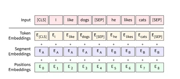
13.3.1 Input Representation
BERT combines three types of embeddings: \[\text{Input}_i = E_{\text{token}}(w_i) + E_{\text{position}}(i) + E_{\text{segment}}(s)\]
1. Token Embeddings
Learned lookup table: \(E_{\text{token}} \in \mathbb{R}^{V \times d}\)
Vocabulary size \(V\) (e.g., 30k), hidden dim \(d\) (768 for BERT-base)
2. Position Embeddings
Learned (not sinusoidal like original Transformer)
\(E_{\text{pos}} \in \mathbb{R}^{L \times d}\) where \(L\) = max sequence length (512)
3. Segment Embeddings
Distinguishes sentence A vs. B (ie., position relative to [SEP] as in [CLS] A [SEP] B [SEP])
\(E_{\text{seg}} \in \mathbb{R}^{2 \times d}\) (only 2 embeddings)
Special Tokens:
[CLS]: Classification token (prepended to sequence)[SEP]: Separator between sentences[MASK]: Masked token for MLM pre-training
13.3.2 Pre-training: Masked Language Modeling
Procedure:
Randomly select 15% of tokens
Of selected tokens: 80% \(\rightarrow\)
[MASK], 10% \(\rightarrow\) random word, 10% \(\rightarrow\) unchangedPredict original token
Loss: \[\mathcal{L}_{\text{MLM}} = -\sum_{i \in \text{selected}} \log P(w_i | w_1, \ldots, [MASK], \ldots, w_n)\]
Why 80/10/10 split?
100%
[MASK]: train/test mismatch (never see[MASK]during fine-tuning)10% random: forces model to use context (can’t just memorize)
10% unchanged: keeps representation of real words
Dynamic Masking: Selection is stochastic and recomputed for each training batch. The same sentence “I love NLP” will have different tokens selected in different epochs:
Epoch 1: mask “love” \(\rightarrow\) “I [MASK] NLP”
Epoch 2: mask “I” \(\rightarrow\) “[MASK] love NLP”
Epoch 3: leave “NLP” unchanged (selected but 10% rule) \(\rightarrow\) “I love NLP”
This prevents overfitting and ensures every token is trained in multiple contexts. Fixed masking would let the model memorize mask positions instead of learning bidirectional representations.
13.3.3 The [CLS] Token: Sentence-Level Representation
The [CLS] token is prepended to every input sequence and serves as an aggregate representation of the entire sequence.
Why [CLS] is important:
Design purpose: Unlike other tokens tied to specific words,
[CLS]has no lexical meaning–it exists solely to aggregate information from all other tokens via self-attentionBidirectional context: Through 12 layers of self-attention, \(h_{\text{[CLS]}}\) attends to all tokens in both directions, capturing sentence-level semantics
Classification head: BERT’s pre-training includes Next Sentence Prediction (NSP) trained on \(h_{\text{[CLS]}}\), making it optimized for sequence-level tasks
Fine-tuning: For downstream classification tasks (sentiment, NLI, QA), add a linear layer on top of \(h_{\text{[CLS]}}\) and fine-tune end-to-end
Key Distinction: While token embeddings \(h_i\) represent individual words in context, \(h_{\text{[CLS]}}\) represents the entire sequence. This makes BERT naturally suited for both token-level tasks (NER, POS tagging) and sequence-level tasks (classification, retrieval).
13.3.4 BERT Output: Extracting Embeddings
Forward pass: \[\begin{align*} & \text{Input: [CLS] I love natural language [SEP]} \\ & \quad \downarrow \\ & \text{Token + Position + Segment embeddings} \\ & \quad \downarrow \\ & \text{12 layers of Self-attention + FFN} \\ & \quad \downarrow \\ & \text{Output: } h_{\text{[CLS]}}, h_{\text{I}}, h_{\text{love}}, h_{\text{natural}}, h_{\text{language}}, h_{\text{[SEP]}} \end{align*}\]
Extracting embeddings:
Sentence-level: Use \(h_{\text{[CLS]}}\) (designed for classification)
Token-level: Use \(h_i\) for token \(i\)
Mean pooling: \(\frac{1}{n}\sum_{i=1}^n h_i\) (average all non-special tokens)
13.4 Modern LLMs: LLaMA, GPT-4
Architecture: Decoder-only transformers (autoregressive LM)
Key Differences from BERT:
Causal attention: Token \(i\) only sees tokens \(1, \ldots, i\) (not future)
Training objective: Next-token prediction (generation), not masked LM
No [CLS] token: No dedicated sequence-level representation
RoPE: Rotary position embeddings (not learned)
Why LLMs are suboptimal for embeddings:
Causal attention limits context (only left-to-right)
Trained for generation, not semantic similarity
Must use ad-hoc pooling (last token, mean-pooling)
14 Dedicated Embedding Models
14.1 Sentence-BERT (SBERT, 2019)
Problem: BERT requires \(O(n^2)\) comparisons
- Comparing 10k sentences: 50M BERT forward passes (intractable)
Solution: Siamese network with contrastive learning
Architecture:
Encode sentence A: \(u = \text{Pool}(\text{BERT}(A))\) (e.g., mean-pool or [CLS] token)
Encode sentence B: \(v = \text{Pool}(\text{BERT}(B))\)
Compare: \(\text{sim}(u, v) = \frac{u^T v}{\|u\| \|v\|}\)
What Gets Trained:
BERT’s weights are fine-tuned (not frozen!)
Pooling has no parameters (just extracts [CLS] or averages token embeddings)
Loss compares sentence embeddings to update BERT such that similar sentences → similar vectors
Base BERT (trained on MLM) doesn’t optimize for sentence similarity; SBERT does
Training Loss (Triplet Loss): \[\mathcal{L} = \max(0, \|u_a - u_p\|^2 - \|u_a - u_n\|^2 + \epsilon)\] where \(u_a\) = anchor, \(u_p\) = positive (similar sentence), \(u_n\) = negative (dissimilar), \(\epsilon\) = margin
Alternative: Contrastive Loss (InfoNCE): \[\mathcal{L} = -\log \frac{\exp(\text{sim}(u_a, u_p) / \tau)}{\exp(\text{sim}(u_a, u_p) / \tau) + \sum_{i=1}^N \exp(\text{sim}(u_a, u_{n_i}) / \tau)}\] Push positive pairs together, negatives apart in embedding space.
Key Insight: Fine-tuning BERT with similarity-based loss (triplet/contrastive) makes embeddings optimized for cosine similarity, unlike base BERT trained on MLM.
Result: Embed once, compare via cosine similarity
Scales to millions of sentences (FAISS, Pinecone)
1000× faster than pairwise BERT comparisons
14.2 Modern Embedding Models (2023+)
Open-source: bge-large, e5-mistral-7b, gte-large, nomic-embed-text
Commercial: OpenAI text-embedding-3, Cohere embed-v3, Voyage AI
Training Improvements:
Hard negative mining: BM25 top-k as hard negatives
In-batch negatives: 511 negatives per example (batch size 512)
Multi-task training: Retrieval, QA, semantic similarity, classification
Matryoshka embeddings: Single model, multiple dimensions
Matryoshka Representation Learning:
\(u \in \mathbb{R}^{1024}\) \(\rightarrow\) can truncate to 768, 512, 256, 128 dims
Training: nested loss at each dimensionality \[\mathcal{L} = \sum_{d \in \{128, 256, 512, 1024\}} \mathcal{L}_d(u[:d])\]
Use case: 128-dim for fast search, 1024-dim for reranking
14.3 ColBERT: Late Interaction
Problem: Mean-pooling loses token-level information
Solution: Keep token embeddings, compute MaxSim score at query time
Architecture:
Query tokens: \(Q = \text{BERT}(q) \in \mathbb{R}^{|q| \times d}\) (e.g., 5 tokens \(\times\) 128 dim)
Document tokens: \(D = \text{BERT}(d) \in \mathbb{R}^{|d| \times d}\) (e.g., 100 tokens \(\times\) 128 dim)
Score: \(\sum_{i=1}^{|q|} \max_{j=1}^{|d|} (Q_i \cdot D_j)\)
Intuition: For each query token, find most similar document token; sum over all query tokens. This captures fine-grained keyword matching while preserving semantic understanding.
Production Implementation:
Offline indexing:
Encode all documents: \(D_i = \text{BERT}(d_i)\) for \(i=1,\ldots,N\)
Store token embeddings in compressed index (e.g., 100 tokens/doc \(\times\) 128 dim)
Build approximate nearest neighbor index (FAISS IVF) for candidate retrieval
Online query:
Encode query: \(Q = \text{BERT}(q)\) (fast, only 5-10 tokens typically)
Candidate retrieval: Use ANN to get top-1000 documents (filter by first-stage similarity)
MaxSim reranking: Compute exact MaxSim score for each of 1000 candidates: \[\text{score}(q, d_i) = \sum_{k=1}^{|q|} \max_{j=1}^{|d_i|} (Q_k \cdot D_{i,j})\]
Return top-K by MaxSim score
Why ColBERT is Slower than SBERT:
| Method | Storage per Doc | Query-time Computation |
|---|---|---|
| SBERT | 1 vector (768 dims) | \(O(1)\) cosine similarity per doc |
| ColBERT | \(\sim\)100 vectors (128 dims each) | \(O(|q| \times |d|)\) MaxSim per doc |
| SBERT total | 768 floats | 768 dot products |
| ColBERT total | 12,800 floats (16\(\times\) larger) | 5 \(\times\) 100 = 500 dot products + max ops |
Concrete Example:
Query: "python async await" (5 tokens)
Document: 100 tokens
SBERT: 1 cosine similarity (768 ops)
ColBERT: For each of 5 query tokens, compute dot product with 100 doc tokens, take max → 5 \(\times\) 100 = 500 dot products + 5 max operations
Even with precomputed doc tokens, MaxSim is \(\sim\)3-5\(\times\) slower per document
For 1M documents: SBERT can use ANN (sublinear); ColBERT needs two-stage (ANN candidates → MaxSim rerank)
When to use ColBERT:
Keyword-heavy retrieval: Code search, technical docs, legal documents
Multi-hop reasoning: Token-level alignment matters (e.g., "red hat" vs "hat" + "red" elsewhere)
Hybrid systems: SBERT for first-pass retrieval (top-10k), ColBERT for reranking (top-100)
Better accuracy: Typically 5-10% improvement over SBERT, at cost of 3-5\(\times\) latency
Optimization Techniques:
Compress doc embeddings to lower dimensions (64 or 32 dims)
Prune document tokens (keep only top-K most salient)
GPU batching for MaxSim computation
Cascade: SBERT (1M→10k) → ColBERT (10k→100) → cross-encoder (100→10)
14.4 Cross-Encoders: Maximum Accuracy
Architecture: Encode query + document together in single BERT pass
How it works: \[\begin{align*} & \text{Input: [CLS] query [SEP] document [SEP]} \\ & \quad \downarrow \\ & \text{BERT encoder (full cross-attention)} \\ & \quad \downarrow \\ & h_{\text{[CLS]}} \rightarrow \text{Classification head} \rightarrow \text{Relevance score} \end{align*}\]
Key difference from bi-encoders (SBERT):
Bi-encoder (SBERT): Encode query and document separately, compare embeddings
score = cosine(embed(query), embed(doc))Pre-compute document embeddings, fast retrieval
Cross-encoder: Encode query + document jointly
score = classifier(BERT([query; doc]))Full attention between query and document tokens
Cannot pre-compute (must encode each pair)
Cross-Encoder Example:
Query: “What is machine learning?”
Document 1: “Machine learning is a subset of AI that enables computers to learn from data.”
Cross-encoder forward pass:
    [CLS] What is machine learning? [SEP]
          Machine learning is a subset... [SEP]
                      ↓
        Self-attention (query tokens attend to doc tokens)
                      ↓
            h_[CLS] → classifier → score = 0.92 (relevant)
Document 2: “The weather today is sunny and warm.”
Cross-encoder forward pass:
    [CLS] What is machine learning? [SEP]
          The weather today... [SEP]
                      ↓
        Self-attention detects semantic mismatch
                      ↓
            h_[CLS] → classifier → score = 0.05 (not relevant)
Why cross-encoders are more accurate:
Token-level interaction: Query word “learning” directly attends to document word “learning”
Full context: Sees both query and document simultaneously
Richer features: 12+ layers of cross-attention
Why cross-encoders are slow:
Cannot pre-compute: each (query, doc) pair needs full BERT pass
Complexity: \(O(n)\) BERT calls for \(n\) documents
Retrieval: 1M documents \(\rightarrow\) hours (vs. seconds for dense retrieval)
Typical RAG pipeline:
| Stage | Method | Candidates | Speed | Accuracy |
|---|---|---|---|---|
| 1. Retrieval | Dense (SBERT) | 1M \(\rightarrow\) 1000 | Fast (ms) | Good |
| 2. Rerank (optional) | ColBERT | 1000 \(\rightarrow\) 100 | Medium | Better |
| 3. Final rerank | Cross-encoder | 100 \(\rightarrow\) 10 | Slow (1s) | Best |
15 Connection to RAG
15.1 RAG Pipeline
1. Indexing Phase: \[\text{Documents} \rightarrow \text{Chunking} \rightarrow \text{Embedding} \rightarrow \text{Vector DB (FAISS/Pinecone)}\]
2. Retrieval Phase: \[\text{Query} \rightarrow \text{Embedding} \rightarrow \text{Similarity Search} \rightarrow \text{Top-K docs}\]
3. Generation Phase: \[\text{Top-K docs + Query} \rightarrow \text{LLM (GPT-4, LLaMA)} \rightarrow \text{Answer}\]
15.2 Embedding Models in RAG
Asymmetric search:
Query: short (5–20 tokens)
Document: long (128–512 tokens)
Need models trained for asymmetric retrieval (
e5-large,bge-large)
Chunking strategies:
Fixed size: 256 tokens with 50-token overlap
Semantic: split by paragraphs, sentences
Hierarchical: summaries + full chunks
15.3 Multi-Stage Retrieval
Two-stage retrieval:
First-pass: Dense retrieval (SBERT) \(\rightarrow\) top-1000
Rerank: ColBERT \(\rightarrow\) top-100
Optional: Cross-encoder \(\rightarrow\) top-10
Trade-off:
Dense: fast, good recall
ColBERT: slower, better precision
Cross-encoder: slowest, best precision
16 Interview Cheat Phrases
TF-IDF to embeddings:
“TF-IDF represents documents as sparse vectors with no semantic similarity. LSA applies SVD to reduce dimensionality, capturing latent topics. Word2Vec replaced this linear factorization with neural networks trained via negative sampling, learning dense embeddings where cosine similarity captures semantics.”
Word2Vec negative sampling:
“Word2Vec skip-gram predicts context from center word. Negative sampling replaces expensive softmax with binary classification: maximize score of positive pairs, minimize score of k negative samples drawn from noise distribution. This is equivalent to implicit factorization of a shifted PMI matrix.”
BERT vs. Word2Vec:
“Word2Vec produces static embeddings–‘bank’ has one vector regardless of context. BERT uses self-attention to create contextualized embeddings where each token’s representation depends on surrounding tokens. This solves polysemy via bidirectional Transformers and MLM pre-training.”
[CLS] token importance:
“The [CLS] token aggregates information from all other tokens through self-attention layers, making it a natural sentence-level representation. BERT’s NSP pre-training optimizes [CLS] for sequence classification, which is why it’s used for embeddings and downstream tasks.”
BERT vs. LLaMA for embeddings:
“BERT’s bidirectional attention and [CLS] token make it naturally suited for embeddings. LLaMA is causal (decoder-only), trained for generation, not similarity. Dedicated embedding models like SBERT, trained with contrastive loss, outperform both for retrieval tasks.”
ColBERT:
“ColBERT keeps token-level embeddings and uses late interaction (MaxSim over all token pairs). This captures fine-grained matching like BM25 while maintaining semantic understanding. It’s used as a reranker in RAG pipelines for precision-critical retrieval.”
Cross-encoder vs. bi-encoder:
“Bi-encoders encode query and document separately, enabling fast retrieval via pre-computed embeddings. Cross-encoders encode them jointly with full cross-attention, achieving higher accuracy but requiring \(O(n)\) forward passes. Use bi-encoders for retrieval, cross-encoders for final reranking.”
Dimensionality reduction:
“PCA finds linear projections via SVD. Neural embeddings learn nonlinear manifolds via gradient descent. Word2Vec with negative sampling implicitly factorizes a PMI matrix but with far more expressive power than PCA.”
17 Summary: Key Takeaways
Evolution: Count-based (TF-IDF) \(\rightarrow\) Matrix factorization (LSA/PCA) \(\rightarrow\) Neural static (Word2Vec/GloVe) \(\rightarrow\) Contextualized (BERT) \(\rightarrow\) Task-optimized (SBERT, BGE)
Word2Vec foundation: Negative sampling made neural embeddings tractable. Understanding this loss function explains the entire embedding paradigm.
Context is critical: Static embeddings fail on polysemy; transformers solve this with self-attention and bidirectional context
Training objective matters: Contrastive loss (SBERT) \(>\) causal LM loss (GPT) for similarity tasks
RAG architecture: Dense retrieval (SBERT) for recall \(\rightarrow\) ColBERT for precision \(\rightarrow\) cross-encoder for final reranking
Modern best practice: Use dedicated embedding models (SBERT, E5, BGE) trained with hard negatives and multi-task objectives. Fine-tune on domain data for 10–20% improvement.
[CLS] token: BERT’s [CLS] token is specifically designed as an aggregate sequence representation through bidirectional self-attention, making BERT naturally suited for embedding tasks unlike causal LLMs.